Generic Example

This example shows how to use calculate the upwelling brigthness temperature by using R16 and R03 absorption model and then plotting them difference.

import matplotlib.pyplot as plt

plt.rcParams.update({'font.size': 15})
import matplotlib.ticker as ticker
from matplotlib.ticker import ScalarFormatter
import numpy as np

Import pyrtlib package

from pyrtlib.climatology import AtmosphericProfiles as atmp
from pyrtlib.tb_spectrum import TbCloudRTE
from pyrtlib.utils import ppmv2gkg, mr2rh

atm = ['Tropical',
       'Midlatitude Summer',
       'Midlatitude Winter',
       'Subarctic Summer',
       'Subarctic Winter',
       'U.S. Standard']

Load standard atmosphere (low res at lower levels, only 1 level within 1 km) and define which absorption model will be used.

z, p, d, t, md = atmp.gl_atm(atmp.TROPICAL)
gkg = ppmv2gkg(md[:, atmp.H2O], atmp.H2O)
rh = mr2rh(p, t, gkg)[0] / 100

mdl = 'R16'

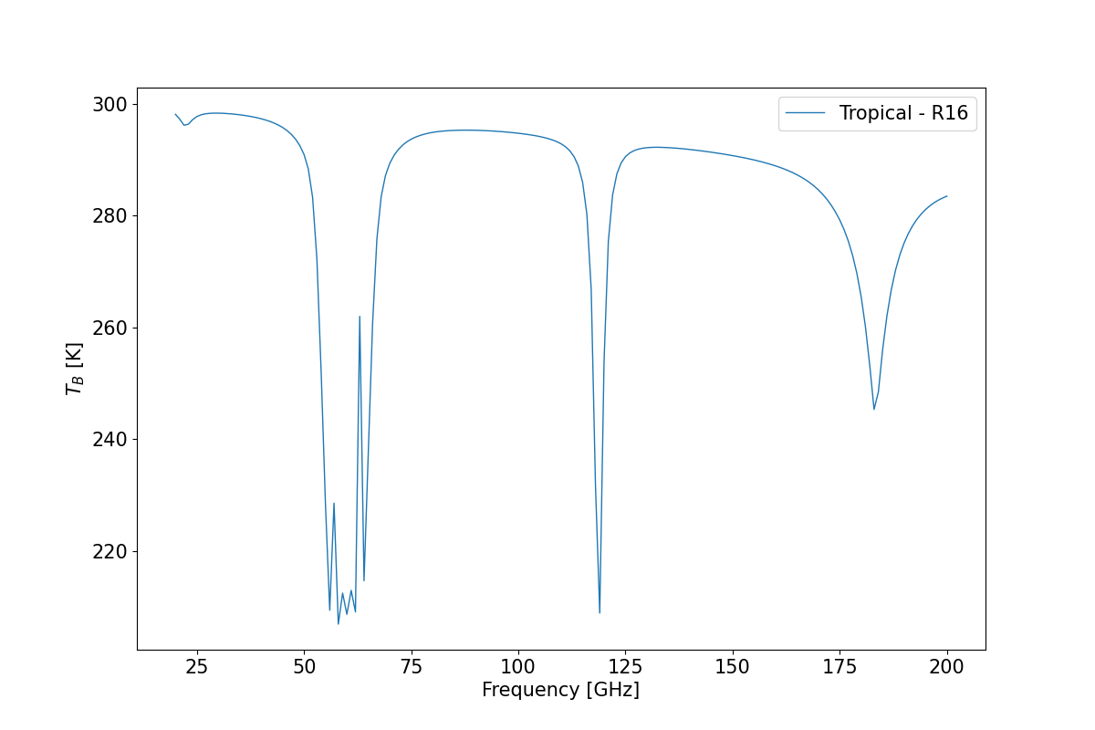
Performing upwelling brightness temperature calculation

Default calculatoin consideres no cloud

ang = np.array([90.])
frq = np.arange(20, 201, 1)
nf = len(frq)

Setup matplotlib plot

fig, ax = plt.subplots(1, 1, figsize=(12,8))
ax.set_xlabel('Frequency [GHz]')
ax.set_ylabel('${T_B}$ [K]')

rte = TbCloudRTE(z, p, t, rh, frq, ang)
rte.init_absmdl(mdl)
df = rte.execute()

df = df.set_index(frq)
df.tbtotal.plot(ax=ax, linewidth=1, label='{} - {}'.format(atm[atmp.TROPICAL], mdl))

ax.legend()
plt.show()

Print dataframe

df

	tbtotal	tbatm	tmr	tmrcld	tauwet	taudry	tauliq	tauice	angle
20	298.109969	0.0	286.950133	0.0	0.120344	0.012855	0.0	0.0	90.0
21	297.245630	0.0	286.301043	0.0	0.188808	0.013524	0.0	0.0	90.0
22	296.153517	0.0	285.000663	0.0	0.261848	0.014259	0.0	0.0	90.0
23	296.340241	0.0	285.636022	0.0	0.257913	0.015066	0.0	0.0	90.0
24	297.158441	0.0	286.738496	0.0	0.202308	0.015954	0.0	0.0	90.0
...	...	...	...	...	...	...	...	...	...
196	281.727042	0.0	281.270840	0.0	3.672975	0.025784	0.0	0.0	90.0
197	282.281780	0.0	281.731501	0.0	3.460000	0.025956	0.0	0.0	90.0
198	282.747798	0.0	282.109277	0.0	3.289848	0.026129	0.0	0.0	90.0
199	283.139746	0.0	282.420450	0.0	3.152710	0.026302	0.0	0.0	90.0
200	283.469554	0.0	282.677693	0.0	3.041424	0.026476	0.0	0.0	90.0

181 rows × 9 columns

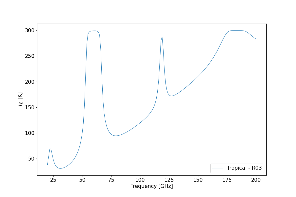
Performing calculation for R03 absorption model

mdl = 'R03'
rte.init_absmdl(mdl)
df_r03 = rte.execute()
df_r03 = df_r03.set_index(frq)

Add brigthness temperature values as new column

df['delta'] = df.tbtotal - df_r03.tbtotal

df

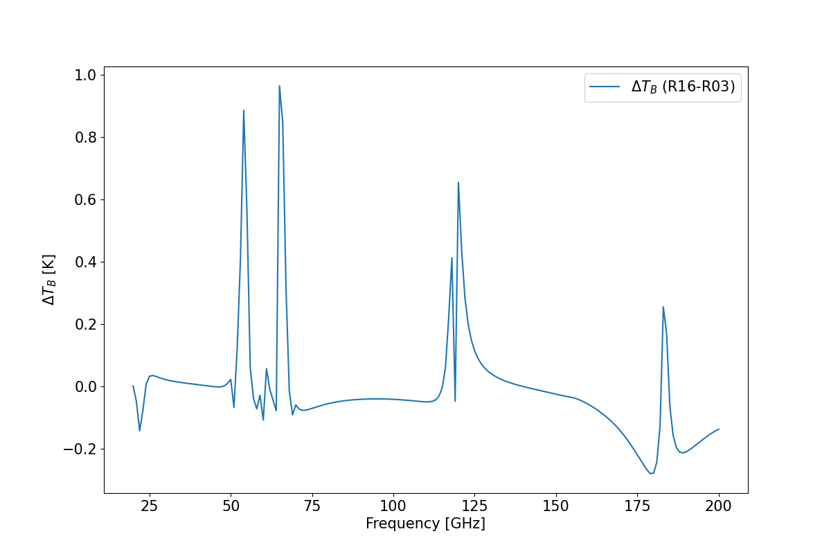
	tbtotal	tbatm	tmr	tmrcld	tauwet	taudry	tauliq	tauice	angle	delta
20	298.109969	0.0	286.950133	0.0	0.120344	0.012855	0.0	0.0	90.0	0.001586
21	297.245630	0.0	286.301043	0.0	0.188808	0.013524	0.0	0.0	90.0	-0.048561
22	296.153517	0.0	285.000663	0.0	0.261848	0.014259	0.0	0.0	90.0	-0.142018
23	296.340241	0.0	285.636022	0.0	0.257913	0.015066	0.0	0.0	90.0	-0.076095
24	297.158441	0.0	286.738496	0.0	0.202308	0.015954	0.0	0.0	90.0	0.007042
...	...	...	...	...	...	...	...	...	...	...
196	281.727042	0.0	281.270840	0.0	3.672975	0.025784	0.0	0.0	90.0	-0.163264
197	282.281780	0.0	281.731501	0.0	3.460000	0.025956	0.0	0.0	90.0	-0.155854
198	282.747798	0.0	282.109277	0.0	3.289848	0.026129	0.0	0.0	90.0	-0.148989
199	283.139746	0.0	282.420450	0.0	3.152710	0.026302	0.0	0.0	90.0	-0.142698
200	283.469554	0.0	282.677693	0.0	3.041424	0.026476	0.0	0.0	90.0	-0.136978

181 rows × 10 columns

Difference between R16 and R03 brightness temperature

fig, ax = plt.subplots(1, 1, figsize=(12,8))
ax.set_xlabel('Frequency [GHz]')
ax.set_ylabel('$\Delta {T_B}$ [K]')
df.delta.plot(ax=ax, figsize=(12,8), label='$\Delta {T_B}$ (R16-R03)')
ax.legend()
plt.show()

Performing downwelling brightness temperature calculation

fig, ax = plt.subplots(1, 1, figsize=(12,8))
ax.set_xlabel('Frequency [GHz]')
ax.set_ylabel('${T_B}$ [K]')

rte.satellite = False
df_from_ground = rte.execute()

df_from_ground = df_from_ground.set_index(frq)
df_from_ground.tbtotal.plot(ax=ax, linewidth=1, label='{} - {}'.format(atm[atmp.TROPICAL], mdl))
ax.legend()
plt.show()

df_from_ground

	tbtotal	tbatm	tmr	tmrcld	tauwet	taudry	tauliq	tauice	angle
20	38.129602	36.135867	287.743834	0.0	0.119654	0.012884	0.0	0.0	90.0
21	53.631602	51.779377	287.523184	0.0	0.183271	0.013539	0.0	0.0	90.0
22	68.663326	66.947486	286.852833	0.0	0.249677	0.014259	0.0	0.0	90.0
23	68.996938	67.298769	287.359400	0.0	0.249866	0.015049	0.0	0.0	90.0
24	58.552279	56.788448	288.054563	0.0	0.201670	0.015918	0.0	0.0	90.0
...	...	...	...	...	...	...	...	...	...
196	290.021111	290.013642	297.081184	0.0	3.697474	0.025231	0.0	0.0	90.0
197	288.153006	288.143908	296.859148	0.0	3.486909	0.025397	0.0	0.0	90.0
198	286.381509	286.370888	296.671344	0.0	3.318905	0.025563	0.0	0.0	90.0
199	284.742973	284.730975	296.513450	0.0	3.183692	0.025730	0.0	0.0	90.0
200	283.257186	283.243976	296.381311	0.0	3.074147	0.025897	0.0	0.0	90.0

181 rows × 9 columns