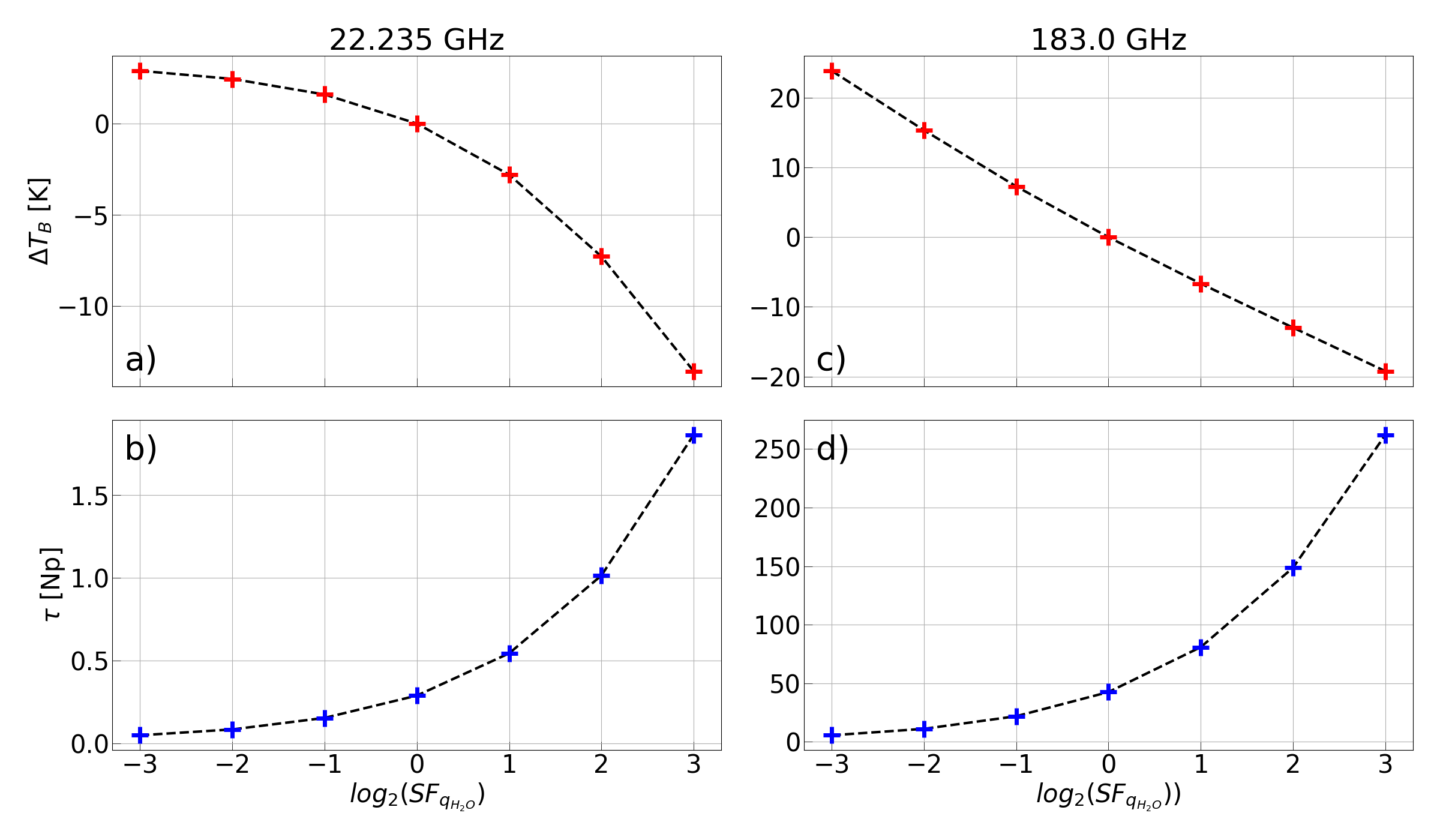
Logarithmic dependence of monochromatic radiance at 22.235 and 183 GHz

This example shows the logarithmic dependence of monochromatic radiance at 22.235 GHz and 183 GHz on the water vapor content in the atmosphere. The brigthness temperature are calculated using the pyrtlib.tb_spectrum.TbCloudRTE method for the zenith view angle and the following water vapor content: 1/8, 1/4, 1/2, 1, 2, 4, 8 times the water vapor content of the reference atmosphere. The reference atmosphere is the Tropical atmosphere

# Reference: Huang & Bani, 2014.

import numpy as np

import matplotlib.pyplot as plt
import matplotlib as mpl
mpl.rcParams["axes.spines.right"] = True
mpl.rcParams["axes.spines.top"] = True
plt.rcParams.update({'font.size': 30})


from pyrtlib.climatology import AtmosphericProfiles as atmp
from pyrtlib.tb_spectrum import TbCloudRTE
from pyrtlib.absorption_model import O2AbsModel
from pyrtlib.utils import ppmv2gkg, mr2rh

z, p, _, t, md = atmp.gl_atm(atmp.TROPICAL)

tb_23 = []
tb_183 = []
tau_23 = []
tau_183 = []
m = [1/8, 1/4, 1/2, 1, 2, 4, 8]

for i in range(0, 7):
    gkg = ppmv2gkg(md[:, atmp.H2O], atmp.H2O) * m[i]
    rh = mr2rh(p, t, gkg)[0] / 100

    # frq = np.arange(20, 201, 1)
    frq = np.array([22.235, 183])
    rte = TbCloudRTE(z, p, t, rh, frq)
    rte.init_absmdl('R22SD')
    O2AbsModel.model = 'R22'
    df = rte.execute()
    df['tau'] = df.tauwet + df.taudry
    tb_23.append(df.tbtotal[0])
    tb_183.append(df.tbtotal[1])
    tau_23.append(df.tau[0])
    tau_183.append(df.tau[1])

tb_023 = np.array(tb_23) - tb_23[3]
tb_0183 = np.array(tb_183) - tb_183[3]

fig, axes = plt.subplots(2, 2, figsize=(24, 14), sharex=True)
axes[0, 1].tick_params(axis='both', direction='in', length=10, width=.5)
axes[0, 1].plot(np.log2(m), tb_0183, linestyle='--', linewidth=3, color='black')
axes[0, 1].plot(np.log2(m), tb_0183, marker='+', linestyle='None', color='r', ms=20, markeredgewidth=5)
axes[0, 1].set_title(f"{frq[1]} GHz")
axes[0, 1].grid(True, 'both')
axes[0, 1].annotate("c)", xy=(0.02, 0.05), xycoords='axes fraction', fontsize=40)

axes[0, 0].set_ylabel('$\Delta T_B$ [K]')
axes[0, 0].tick_params(axis='both', direction='in', length=10, width=.5)
axes[0, 0].plot(np.log2(m), tb_023, linestyle='--', linewidth=3, color='black')
axes[0, 0].plot(np.log2(m), tb_023, marker='+', linestyle='None', color='r', ms=20, markeredgewidth=5)
axes[0, 0].set_title(f"{frq[0]} GHz")
axes[0, 0].grid(True, 'both')
axes[0, 0].annotate("a)", xy=(0.02, 0.05), xycoords='axes fraction', fontsize=40)

axes[1, 1].set_xlabel('$log_2(SF_{q_{H_2O}}))$')
axes[1, 1].tick_params(axis='both', direction='in', length=10, width=.5)
axes[1, 1].plot(np.log2(m), tau_183, linestyle='--', linewidth=3, color='black')
axes[1, 1].plot(np.log2(m), tau_183, marker='+', linestyle='None', color='blue', ms=20, markeredgewidth=5)
axes[1, 1].grid(True, 'both')
axes[1, 1].annotate("d)", xy=(0.02, 0.88), xycoords='axes fraction', fontsize=40)

axes[1, 0].set_xlabel('$log_2(SF_{q_{H_2O}})$')
axes[1, 0].set_ylabel('$\\tau$ [Np]')
axes[1, 0].tick_params(axis='both', direction='in', length=10, width=.5)
axes[1, 0].plot(np.log2(m), tau_23, linestyle='--', linewidth=3, color='black')
axes[1, 0].plot(np.log2(m), tau_23, marker='+', linestyle='None', color='blue', ms=20, markeredgewidth=5)
axes[1, 0].grid(True, 'both')
axes[1, 0].annotate("b)", xy=(0.02, 0.88), xycoords='axes fraction', fontsize=40)

plt.tight_layout()

plt.show()